
Next-generation sequencing (NGS) enables high-throughput detection of DNA sequences in genomic research. The NGS technologies are implemented for several applications, including whole-genome sequencing, de novo assembly sequencing, resequencing, and transcriptome sequencing at the DNA or RNA level. In order to sequence longer sections of DNA, a new approach called shotgun sequencing (Venter et al., 2003; Margulies et al., 2005; Shendure et al., 2005) was developed during Human Genome Project (HGP). In this approach, genomic DNA is enzymatically or mechanically broken down into smaller fragments and cloned into sequencing vectors in which cloned DNA fragments can be sequenced individually. Detecting abnormalities across the entire genome (whole-genome sequencing only), including substitutions, deletions, insertions, duplications, copy number changes (gene and exon) and chromosome inversions/translocations are possible with the help of the NGS approach. Thus, shotgun sequencing has more significant advantages from the original sequencing methodology, Sanger sequencing, that requires a specific primer to start the read at a specific location along with the DNA template and record the different labels for each nucleotide within the sequence.
The aim of this study is to build a general workflow of mapping the short-read sequences that came from NGS machine.
Before the analysis of NGS data with publicly or commercially available algorithms and tools, we need to know about some features of the NGS raw data.
The raw data from a sequencing machine are most widely provided as FASTQ (unaligned sequences) files, which include sequence information, similar to FASTA files, but additionally contain further information, including sequence quality information. A FASTQ file consists of blocks, corresponding to reads, and each block consists of four elements in four lines.
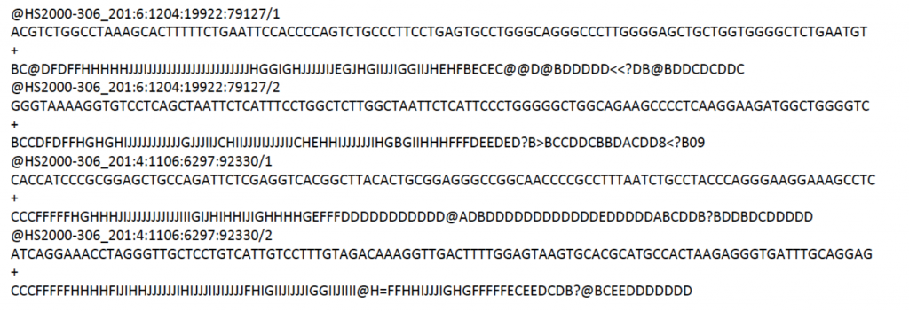
Line 1 begins with a ‘@’ character and is followed by a sequence identifier and an optional description
Line 2 is the raw sequence letters
Line 3 begins with a ‘+’ character and is optionally followed by the same sequence identifier (and any description) again
Line 4 encodes the quality values for the sequence in Line 2, and must contain the same number of symbols as letters in the sequence
For instance;
@HS2000-306_201:6:1204:19922:79127/
| Column | Brief Description |
| HS2000-306_21 | The instrument name |
| 6 | Flowcell lane |
| 1204 | Tile number within the flowcell lane |
| 19922 | x-coordinate of the cluster within the tile |
| 79127 | y-coordinate of the cluster within the tile |
| 1 | the member of a pair, 1 or 2 (paired-end) |
ACGTCTGGCCTAAAGCACTTTTTCTGAATTC… Sequence
+
BC@DFDFFHHHHHJJJIJJJJJJJJJJJJJJJJJJJJJH… Base Qualities
1.Quality Control
Quality control is the most important step in the process of improving raw data by removing any identifiable errors from it. With the application of QC at the beginning of the analysis, the chance of finding any contamination, imprecision, error, and missing data are reduced.
Quality (Q) is proportional to -log10 probability of sequence base being wrong (e):
Phred scaled Q = -10*log10(e)
Base Qualities = ASCII 33 + Phred scaled Q
e: base-calling error probability
SAM encoding adds 33 to the value because ASCII 33 is the first visible character.
Phred Quality Score | Probability of Incorrect Base Call | Base Call Accuracy |
| 10 | 1 in 10 | 90% |
| 20 | 1 in 100 | 99% |
| 30 | 1 in 1000 | 99.9% |
| 40 | 1 in 10,000 | 99.99% |
| 50 | 1 in 100,000 | 99.999% |
| 60 | 1 in 1,000,000 | 99.9999% |
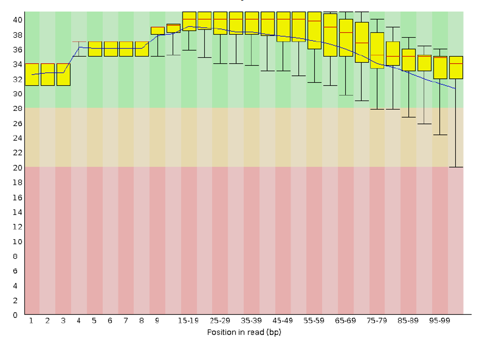
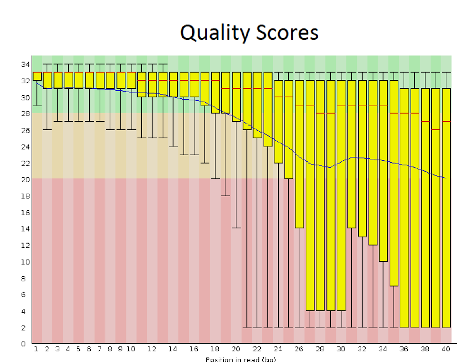
The most commonly used tool for assessing and visualizing the quality of FASTQ data is FastQC (Babraham Bioinformatics, n.d.), which provides comprehensive information about data quality, including base sequence quality scores, GC content information, sequence duplication levels, and overrepresented sequences. There are some alternatives to FastQC, and these are PRINSEQ, fastqp, NGS QC Toolkit, and QC-Chain
Running FastQC
1- To run the FastQC program on desktop, you can use File > Open to select the sequence file you want to check.
2- To run the FastQC program in the cluster, we would normally have to tell our computer where the program is located.
$ which fastqc
/usr/local/bin/fastqc
FastQC can accept multiple filenames as input, so we can use the *.fastq.gz wildcard to run FastQC on all of the FASTQ files in this directory.
$ fastqc *.fastq.gz
You will see an automatically updating output message telling you the progress of the analysis. It will start like this:
Started analysis of SRR2584863_1.fastq
Approx 5% complete for SRR2584687_1.fastq
Approx 10% complete for SRR2584687_1.fastq
Approx 15% complete for SRR2584687_1.fastq
Approx 20% complete for SRR2584687_1.fastq
Approx 25% complete for SRR2584687_1.fastq
Approx 30% complete for SRR2584687_1.fastq
Approx 35% complete for SRR2584687_1.fastq
Approx 40% complete for SRR2584687_1.fastq
Approx 45% complete for SRR2584687_1.fastq
For each input FASTQ file, FastQC has created a .zip file and a .html file. The .zip file extension indicates that this is actually a compressed set of multiple output files. We’ll be working with these output files soon. The .html file is a stable webpage displaying the summary report for each of our samples.
We want to keep our data files and our results files separate, so we will move these output files into a new directory within our results/ directory. If this directory does not exist, we will have to create it.
## -p flag stops a message from appearing if the directory already exists
$ mkdir -p ~/kaya/ results
$ mv *.html ~/kaya/ results/
$ mv *.zip ~/kaya/ results/
It can be quite tedious to click through multiple QC reports and compare the results for different samples. It is useful to have all the QC plots on the same page so that we can more easily spot trends in the data.
The .html files and the uncompressed .zip files are still present, but now we also have a new directory for each of our samples. We can see for sure that it’s a directory if we use the -F flag for ls.
$ ls -F
SRR2584869_1_fastqc/ SRR2584866_1_fastqc/ SRR2589044_1_fastqc/SRR2584869_1_fastqc.html SRR2584866_1_fastqc.html SRR2589044_1_fastqc.htmlSRR2584863_1_fastqc.zip SRR2584866_1_fastqc.zip SRR2589044_1_fastqc.zipSRR2584863_2_fastqc/ SRR2584866_2_fastqc/ SRR2589044_2_fastqc/SRR2584863_2_fastqc.html SRR2584866_2_fastqc.html SRR2589044_2_fastqc.htmlSRR2584863_2_fastqc.zip SRR2584866_2_fastqc.zip SRR2589044_2_fastqc.zip
Let’s see what files are present within one of these output directories.
$ ls -F SRR2584869_1_fastqc/
fastqc_data.txt fastqc.fo fastqc_report.html Icons/ Images/ summary.txt
Use less to preview the summary.txt file for this sample.
$ less SRR2584869_1_fastqc/summary.txt
PASS Basic Statistics SRR2584869_1.fastq
PASS Per base sequence quality SRR2584869_1.fastq
PASS Per tile sequence quality SRR2584869_1.fastq
PASS Per sequence quality scores SRR2584869_1.fastq
WARN Per base sequence content SRR2584869_1.fastq
WARN Per sequence GC content SRR2584869_1.fastq
PASS Per base N content SRR2584869_1.fastq
PASS Sequence Length Distribution SRR2584869_1.fastq
PASS Sequence Duplication Levels SRR2584869_1.fastq
PASS Overrepresented sequences SRR2584869_1.fastq
WARN Adapter Content SRR25848
Finally, we can make a report of the results we got for all our samples by concatenating all of our summary.txt files into a single file using the cat command.
$ cat */summary.txt > ~/kaya/results/fastqc_summaries.txt
For more information, please see the FastQC documentation here
Additionally, the multiqc tool has been designed for the tasks of combining QC reports into a single report that is easy to analyze
$multiqc
$multiqc –help
Another way to check your NGS data quality is to work in R studio.
fastqcr can be installed from CRAN as follow.
install.packages(“fasqcr”)
2. Trimming Low-quality Reads and Adapters
Trimming is the second step in analyzing NGS data. It has been broadly embraced in most recent NGS studies, specifically prior to genome assembly, transcriptome assembly, metagenome reconstruction, gene expression, epigenetic studies, and comparative genomics. Neglecting the presence of low-quality base calls may, in fact, be harmful to any NGS analysis, as it may add unreliable and potentially random sequences to the dataset. This may constitute a relevant problem for any downstream analysis pipeline and lead to false definitions of data. Also, adapter contamination can lead to NGS alignment errors and an increased number of unaligned reads, since the adapter sequences are synthetic and do not occur in the genomic sequence. There are applications (e.g., small RNA sequencing) where adapter trimming is highly necessary. With a fragment size of around 24 nucleotides, one will definitely sequence into the 3′ adapter. But there are also some applications (transcriptome sequencing, whole-genome sequencing, etc.) where adapter contamination can be expected to be so small (due to an appropriate size selection) that one could consider to skip the adapter removal and thereby save time and efforts. There are many tools to handle of QC, namely, AfterQc, Cutadapt, Trimmomatic, Erne-Filter, ConDeTri, Sickle, SolexaQA, AlienTrimmer, Skewer , BBDuk, Fastx Toolkit, and Trim Galore.
In the present work, we want to describe the basic commands to improve your NGS data quality and authenticity by the Cutadapt trimming tool.
When processing paired-end data, Cutadapt holds the trimming these reads. To facilitate this, provide two input files and a second output file with the -p option (this is the short form of –paired-output). This is the basic command-line syntax:
$ cutadapt -a ADAPTER_FWD -A ADAPTER_REV -o out.1.fastq -p out.2.fastq reads.1.fastq reads.2.
Here, the input reads are in reads.1.fastq and reads.2.fastq, and the result will be written to out.1.fastq and out.2.fastq.
In paired-end mode, the options -a, -b, -g and -u that also exist in single-end mode are applied to the forward reads only. To modify the reverse read, these options have uppercase versions -A, -B, -G and -U that work just like their counterparts. In the example above, ADAPTER_FWD will therefore be trimmed from the forward reads and ADAPTER_REV from the reverse reads.
The -q (or –quality-cutoff) parameter can be used to trim low-quality ends from reads. If you specify a single cutoff value, the 3’ end of each read is trimmed:
$ cutadapt -q 20,20 -o output.fastq input.fastq
It is also possible to also trim from the 5’ end by specifying two comma-separated cutoffs as 5’ cutoff, 3’ cutoff. For example,
$ cutadapt -q 15,10 -o output.fastq input.fastq
will quality-trim the 5’ end with a cutoff of 15 and the 3’ end with a cutoff of 10. To only trim the 5’ end, use a cutoff of 0 for the 3’ end, as in -q 15,0.
Interleaved paired-end reads
Paired-end reads can be read from a single FASTQ file in which the entries for the first and second read from each pair alternate. The first read in each pair comes before the second. Enable this file format by adding the –interleaved option to the command-line. For example:
$ cutadapt –interleaved -q 20 -a ACGT -A TGCA -o trimmed.fastq reads.fastq
To read from an interleaved file, but write regular two-file output, provide the second output file as usual with the -p option:
$ cutadapt –interleaved -q 20 -a ACGT -A TGCA -o trimmed.1.fastq -p trimmed.2.fastq reads.fastq
Reading two-file input and writing interleaved is also possible by providing a second input file:
$ cutadapt –interleaved -q 20 -a ACGT -A TGCA -o trimmed.1.fastq reads.1.fastq reads.2.fas
Trimming paired-end reads separately
Secondly, if you want to quality-trim the first read in each pair with a threshold of 20, and the second read in each pair with a threshold of 10, then the commands could be:
$ cutadapt -q 20 -a ADAPTER_FWD -o trimmed.1.fastq reads1.fastq
$ cutadapt -q 10 -a ADAPTER_REV -o trimmed.2.fastq reads2.fastq
If one end of a paired-end read had > 5 % ‘N’ bases, then the paired-end read can be removed. To deal with, Cutadapt recommends the following options to deal with N bases in your reads:
–max-n COUNT
Discard reads containing more than COUNT N bases. A fractional COUNT between 0 and 1 can also be given and will be treated as the proportion of maximally allowed N bases in the read.
–trim-n
Remove flanking N bases from each read. That is, a read such as this:
NNACGTACGTNNNN
It trimmed to just Ns and the rest of the sequence became ACGTACGT. This option is applied after adapter trimming. If you want to get rid of N bases before adapter removal, use quality trimming: N bases typically also have a low quality value associated with them.
Finally, Cutadapt has two sets of adapters to work with:
An example:
$ cutadapt –pair-adapters -a AAAAA -a GGGG -A CCCCC -A TTTT -o out.1.fastq -p out.2.fastq in.1.fastq in.2.fastq
Here, the adapter pairs are (AAAAA, CCCCC) and (GGGG, TTTT). That is, paired-end reads will only be trimmed if either
- AAAAA is found in R1 and CCCCC is found in R2,
- or GGGG is found in R1 and TTTT is found in R2.
For detailed information, please see the Cutadapt documentation.
3. Aligned sequences – SAM/BAM format
Now, filtered reads of each sequencing sample are ready to attain the exact locations onto the corresponding reference genome. Also, you can find these locations using de novo assembly.
A reference genome is a collection of contigs
● A contig refers to overlapping DNA reads encoded as A, G, C, T or N
● Typically comes in FASTA format:
○ “>” line contains information on contig
There are a number of tools to choose from and, while there is no golden rule, there are some tools that are better suited for particular NGS analyses, to name a few, BWA, Bowtie2, SOAP, novoalign, and mummer. After aligning, a Sequence Alignment Map (SAM) file is produced. This file is a format for storing large nucleotide sequence alignments. The binary version of a SAM file is termed a Binary Alignment Map (BAM) file, and BAM file stores aligned reads and are technology independent. The SAM/BAM file consists of a header and an alignment section.
We will be using the Burrows Wheeler Aligner (BWA), which is a software package for mapping short-read sequences against a reference genome.
The alignment process consists of two steps:
- Indexing the reference genome
- Aligning the reads to the reference genome
Firstly, we create a new folder and download our reference genome from our source.
$ cd ~/kaya
$ mkdir -p data/ref_genome
$ curl -L -o data/ref_genome/ecoli_ref.fasta.gz ftp://ftp.ncbi.nlm.nih.gov/genomes/all/GCA/000/017/985/GCA_000017985.1_ASM1798v1/GCA_000017985.1_ASM1798v1_genomic.fna.gz
$ gunzip data/ref_genome/ecoli_ref.fasta.gz
We will also download a set of trimmed FASTQ files to work with.
$ curl -L -o sub.tar.gz https://ndownloader.figshare.com/files/14418248
$ tar xvf sub.tar.gz
$ mv sub/ ~/kaya/data/trimmed_fastq_small
and you need to create multiple directories for the results that will be generated as part of this workflow.
$ mkdir -p results/sam_results/bam_results
Index the reference genome
Our first step is to index the reference genome for use by BWA. Indexing allows the aligner to quickly find potential alignment sites for query sequences in a genome, which saves time during alignment. Indexing the reference only has to be run once. The only reason you would want to create a new index is if you are working with a different reference genome or you are using a different tool for alignment.
$ bwa index data/ref_genome/ecoli_ref.fasta
## While the index is created, you will see output that looks something like this:
[bwa_index] Pack FASTA… 0.04 sec
[bwa_index] Construct BWT for the packed sequence…
[bwa_index] 1.05 seconds elapse.
[bwa_index] Update BWT… 0.03 sec
[bwa_index] Pack forward-only FASTA… 0.02 sec
[bwa_index] Construct SA from BWT and Occ… 0.57 sec
[main] Version: 0.7.17-r1188
[main] CMD: bwa index data/ref_genome/ecoli_rel606.fasta
[main] Real time: 1.765 sec; CPU: 1.715 sec
Align reads to reference genome
The alignment process consists of choosing a suitable reference genome to map our reads against and then choosing on an aligner. We will use the BWA-MEM algorithm, which is the latest and is generally recommended for high-quality queries as it is faster and more accurate.
An example of what a bwa command looks like is below. This command will not run, as we do not have the files ref_genome.fa, input_file_R1.fastq, or input_file_R2.fastq.
$ bwa mem ref_genome.fasta input_file_R1.fastq input_file_R2.fastq > output.sam
We are running bwa with the default parameters here, your use case might require a change of parameters. NOTE: Always read the manual page for any tool before using and make sure the options you use are appropriate for your data.
We’re going to start by aligning the reads from just one of the samples in our dataset (SRR2584687). Later, we’ll be iterating this whole process on all of our sample files.
$ bwa mem data/ref_genome/ecoli_ref.fasta data/trimmed_fastq_small/SRR2584687_1.trim.sub.fastq data/trimmed_fastq_small/SRR2584687_2.trim.sub.fastq > results/sam/SRR2584687.aligned.sam
##You will see output that starts like this:
[M::bwa_idx_load_from_disk] read 0 ALT contigs
[M::process] read 77446 sequences (10000033 bp)…
[M::process] read 77296 sequences (10000182 bp)…
[M::mem_pestat] # candidate unique pairs for (FF, FR, RF, RR): (48, 36728, 21, 61)
[M::mem_pestat] analyzing insert size distribution for orientation FF…
[M::mem_pestat] (25, 50, 75) percentile: (420, 660, 1774)
[M::mem_pestat] low and high boundaries for computing mean and std.dev: (1, 4482)
[M::mem_pestat] mean and std.dev: (784.68, 700.87)
[M::mem_pestat] low and high boundaries for proper pairs: (1, 5836)
[M::mem_pestat] analyzing insert size distribution for orientation FR…
SAM/BAM format
The SAM file, is a tab-delimited text file that contains information for each individual read and its alignment to the genome.
The compressed binary version of SAM is called a BAM file. We use this version to reduce size and to allow for indexing, which enables efficient random access of the data contained within the file.
The file begins with a header, which can be optional. The header is used to describe the source of data, a reference sequence, method of alignment, etc., this will change depending on the aligner being used. Following the header is the alignment section. Each line that follows corresponds to alignment information for a single read. Each alignment line has 11 necessary fields for essential mapping information and a variable number of other fields for aligner specific information. An example entry from a SAM file is displayed below with the different fields highlighted.
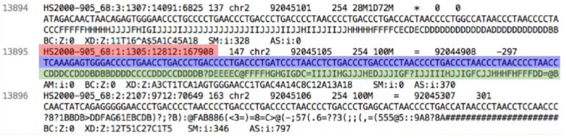
The sequence of Read (BLUE)
Encoded Sequence Quality (GREEN)

(POS) Position in chromosome to which 5′ end of the read aligns
Alignment information – “Cigar string” (BLUE)
100M – Continuous match of 100 bases (perfect match or mismatch)
28M1D72M – 28 bases continuously match, 1 deletion from reference, 72 base match (GREEN)
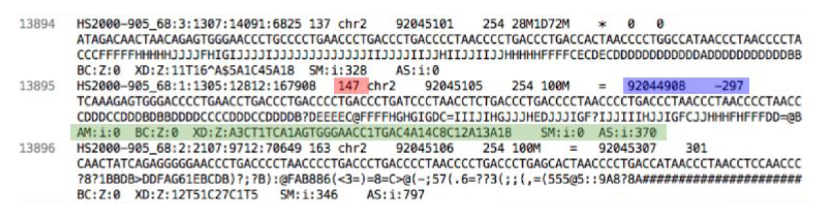
(BLUE) -ISIZE- Paired read position and insert size
(GREEN) User defined flags
We will convert the SAM file to BAM format using the samtools program with the view command and tell this command that the input is in SAM format (-S) and to output BAM format (-b):
$ samtools view -S -b results/sam/SRR2584687.aligned.sam > results/bam/SRR2584687.aligned.
Sort BAM file by coordinates
Next, we sort the BAM file using the sort command from samtools. -o tells the command where to write the output.
$ samtools sort -o results/bam/SRR2584687.aligned.sorted.bam results/bam/SRR2584687.aligned.bam
If you want to follow statistics about your sorted bam file:
$ samtools flagstat results/bam/SRR2584687.aligned.sorted.bam
#OUPUT
231341 + 0 in total (QC-passed reads + QC-failed reads)
0 + 0 secondary
1169 + 0 supplementary
0 + 0 duplicates
351103 + 0 mapped (99.98% : N/A)
350000 + 0 paired in sequencing
175000 + 0 read1
175000 + 0 read2
346688 + 0 properly paired (99.05% : N/A)
349876 + 0 with itself and mate mapped
58 + 0 singletons (0.02% : N/A)
0 + 0 with mate mapped to a different
chr0 + 0 with mate mapped to a different chr (mapQ>=5)
v2- Align the reads to the contigs using BWA
$bwa index kaya/LS0566-contigs.fa
$bwa mem -t2 kaya/LS0566-contigs.fa 25KLUK_4_1.fq.gz 25KLUK_4_2.fq.gz >kaya/25KLUK_4.sam
$samtools sort -@2 -o kaya/25KLUK_4.bam kaya/25KLUK_4.sam
$samtools index kaya/25KLUK_4.bam
Index the assembly FASTA file.
$ samtools faidx kaya/LS0566-contigs.fa
Viewing BAM file using samtools tview.
$ samtools tview kaya/25KLUK_4.bam kaya/LS0566-contigs.fa
You can browse your BAM file with IGV
4. Viewing with IGV
IGV is a genome browser, which has the advantage of being installed locally and providing fast access. Web-based genome browsers, like Ensembl or the UCSC browser, are slower but provide more functionality.
Locally on your own Mac or Windows computer
We need to open the IGV software. If you haven’t done so already, you can download IGV from the Broad Institute’s software page, double-click the .zip file to unzip it, and then drag the program into your Applications folder.
- Open IGV.
- Load our reference genome file (ecoli_ref.fasta) into IGV using the “Load Genomes from File…“ option under the “Genomes” pull-down menu.
Load our BAM file (SRR2584687.aligned.sorted.bam) using the “Load from File…“ option under the “File” pull-down menu.
To load data from an HTTP URL:
- Select File>Load from URL.
- Enter the HTTP or FTP URL for a data file or sample information file.
- If the file is indexed, enter the index file name in the field provided.
- Click OK.
To load a file from Google Cloud Storage, enter the path to the file with the “gs://” prefix. //
Upload the following indexed/sorted Bam files with File -> Load from URL >http://faculty.xxx.edu/~kaya/Workshop/results/SRR20372154.fastq.bam
Controlling IGV from R
You can open IGV from within R with startIGV(“lm”) . Note this may not work on all systems. The testing URL (xxx.edu) is given below. You can try with your cluster URL.
library(SRAdb)
urls <- readLines(“http://xxxx.edu/data/samples/bam_urls.txt“)
#startIGV(“lm”) # opens IGV
sockiv <- IGVsocket()
session <- IGVsession (files=urls,
sessionFile=“session.xml”,
genome=“A. thaliana (TAIR10)”)
IGVload(sockiv, session)
IGVgoto(sockiv, ‘Chr2:67296-3521’)
I hope you find this tutorial useful to analyze your NGS data.
I would like to thank Dilek Koptekin ( @dilekopter ) for reviewing the pipeline. If you have any questions, please get in touch with us without hesitation.
References
Brabaham Bioinformatics website. Available: http:// www.bioinformatics.babraham.ac.uk/projects/fastqc/. Accessed 2013 Dec 1
Cock PJ, Fields CJ, Goto N, Heuer ML, Rice PM (2010) The Sanger FASTQ file format for sequences with quality scores, and the Solexa/ Illumina FASTQ variants. Nucleic Acids Res 38: 1767-1771. doi: 10.1093/nar/gkp1137. PubMed: 20015970.
Del Fabbro C, Scalabrin S, Morgante M, Giorgi FM (2013) An Extensive Evaluation of Read Trimming Effects on Illumina NGS Data Analysis. PLoS ONE 8(12): e85024. doi:10.1371/journal.pone.0085024
Martin M (2011) Cutadapt removes adapter sequences from high- throughput sequencing reads. EmBnet Journal 17: 10-12.
Zhang J, Chiodini R, Badr A, Zhang G. The impact of next-generation sequencing on genomics. J Genet Genomics. 2011;38(3):95–109. doi:10.1016/j.jgg.2011.02.003