qPCR Primer Design Tutorial

(The original tutorial I prepared with Microsoft Sway last year can be found here.)

PCR (Polymerase Chain Reaction) is a method widely used in the wet-lab to amplify the specific target sequences (mostly either directly from DNA or converting messenger RNA/mRNA to cDNA, then amplification of the target, also known as RT-PCR).

Nowadays, it is also popular among public due to accuracy of the detection for the viral materials during SARS-COV-2 caused pandemic (COVID, for more information, click here.).

Brief History of the Discovery of PCR

Shortly after the synthesis of oligonucleotides synthetically in the lab, young scientist Karry B. Mullis was curious about making more copies of scarce genetic materials for further studies. The question was “but how?”. In fact, this milestone technology was rewarded by Nobel Prize (in Chemistry at 1993. For more information, click here.).

Advantages of PCR

• It reproduces accurate millions of copies of a given target in a short period of time by taking advantage of extremely heat resistant (in contrast to human enzymes) Taq DNA polymerase of thermophilic (=heat lover) bacteria.
• It enables identification and modification of genetic materials.

RT-qPCR is real-time, quantitative and reverse-transcribed nucleic acid such as transcripts, version of regular PCR, which enables the simultaneous surveillance of amplification during the cycles thanks to fluorescent dye/probes.

It shares the similar steps with regular PCR: denaturation, annealing and elongation.

How to amplify?

Apart from the DNA polymerase (the enzyme), suitable buffer for the enzyme and the target nucleic acid sequence, it is required to have a proper primer sequences (forward and reverse) for DNA polymerase to bind and reproduce the target area on the sequence.

Primer pairs do not only provide a docking and start site for the enzyme, but also provide the determination of target site. Thus, it is important to design primers properly. It usually preferred as 15-25 nucleotides (denoted as nt) long single stranded DNA sequences (optimizing the trade-off between cost and specificity).

Here, we will learn how to design a qPCR primer for a target sequence and how to analyze the data in the following slides.

Main objectives of the tutorial course are:

1. Understanding the importance of q/PCR for biology
2. Learn the basics for primer design for qPCR
3. Introduction to NCBI
4. Primer design: using NCBI-PrimerBLAST
5. Primer design: using Primer3
6. Importance of In Silico testing of primers
7. In Silico PCR
8. Learning about qPCR analysis: Reference Gene
9. Learning about qPCR analysis: qPCR Data Analysis
10. Additional notes about primer efficiency calculation and tissue specific expression

Using NCBI to find the detailed information about the target gene

NCBI is the website of National Center for Biotechnology and Information hosted by US Government and open to everyone. It has many useful features including Pubmed, BLAST , SRA for sequence data archiving and more. Today, we will focus on Gene and PrimerBLAST features.

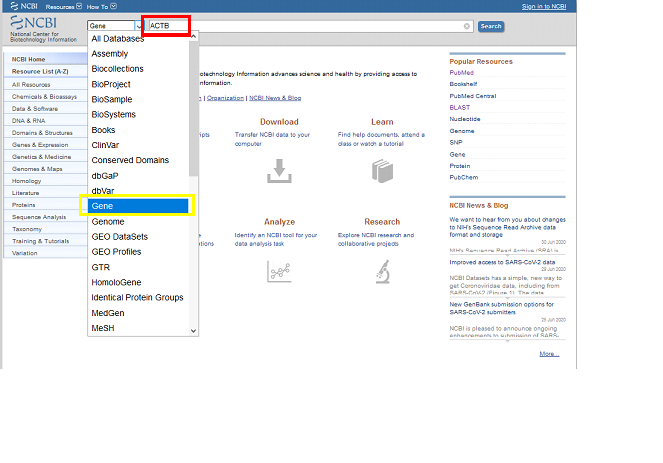
Type the target (gene) name to the NCBI“Search” box. For the sake of this tutorial, let’s continue with “ACTB” as the target. Search under “Gene” category on the left.

You will see different options after click search. These are either the corresponding human ACTB gene in other species (defined as “ortholog“), or the duplicates of the genes happened in the evolution history of the gene in the same specie having difference in the sequence and/or function (defined as “paralog“, for more information, please use this link).

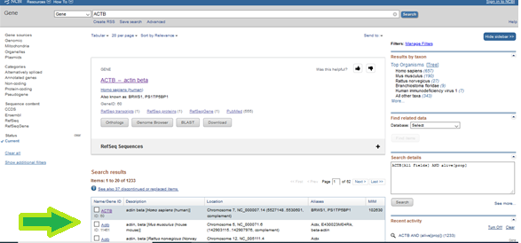
You can find various information about the target gene here. To exemplify, exonic-intronic regions, the chromosome where the gene is located, which tissue(s) it is expressed in the Expression part, or the phenotypic relationship, single nucleotide variations (SNPs) and more (UCSC Genome Browser can be an alternative tool to use at this point.)

When you scroll down little bit, you can see all the transcripts (the expressed RNA) of the relevant gene.

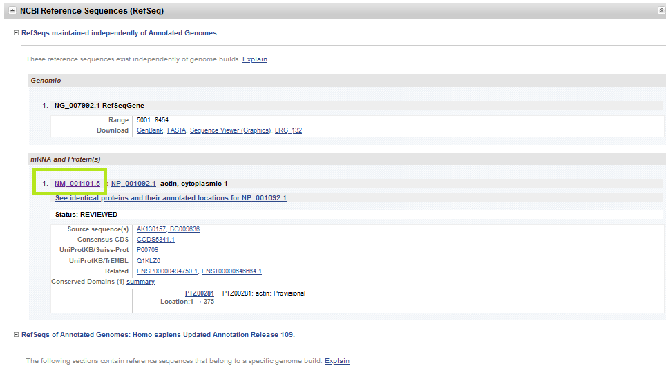
Let’s see the details of relevant mRNA of the gene simply from NCBI-Nucleotide instead of NCBI-Gene (there is more than one way of reaching the information).

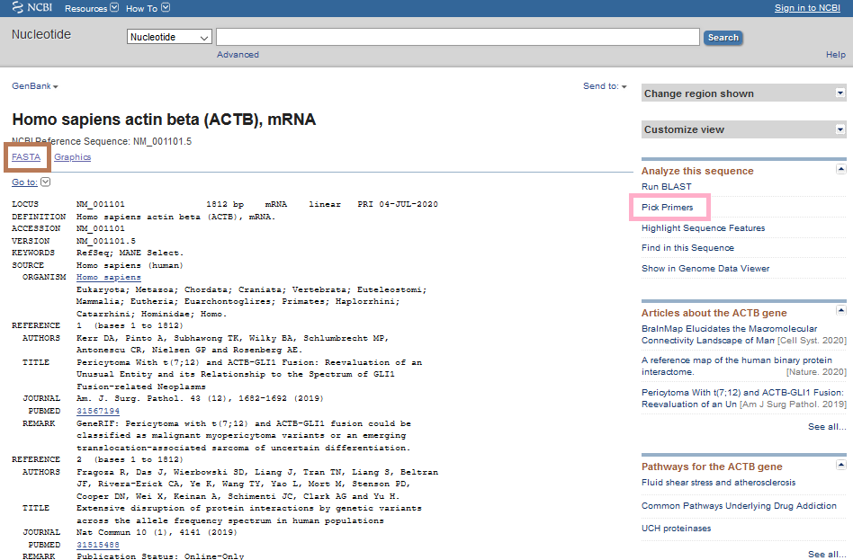
There are two options here. The first option is the one shown with pink color: Pick Primers. This directs you to Primer-BLAST to design primers. The second option shown in brown box leads you to FASTA sequence (the nucleotides in A, T, C, G format). You can copy and paste the sequence in FASTA format in alternative primer design tools such as Primer3. Let’s see the options in detail.

Primer-BLAST

If you have chosen “Pick Primer”, this will lead you to the page below:

Now, you can change the parameters about your primer here. You can use the the boxes with question mark on the right to learn more about the details of the parameters.

Let’s look at some of them in detail.

• PCR product size given in red box, shows the length of the target area you want to amplify. If you are interested in specific transcripts of the gene, you might not need to amplify the whole sequence.

In this case, it is better to take the optimal and maximum length of the target that SYBR-Green (in this case, fluorescent dye that interacts with double stranded-DNA, also known as ds-DNA, and gives the signal to help quantification). Although 500 base pair (denoted as bp) has given as the maximum detection limit for the qPCR target, it usually works in optimum for 100-200 nt target.

• You can use # of primers to return given in orange box to set the number of primer pairs that you want to return (e.g. show me most suitable top 10)
• Usually we use both forward and reverse primers to amplify the target. It is important these primers to have similar melting temperature, Tm (which is used to set annealing temperature). You can adjust this by using the box in blue (e.g. show me the primer pairs having at least 57 and at most 63 Tm, having the difference at most 3 degree between each).
• If you are not sure about your purpose, it is better stay spanning exon exon junction shown in green box (you can find the details here.)
• You can see the parameters in a new window by selecting “show results in a separate window” , which helps you to save some time if you need to change the parameters.

You can always use “advanced parameters” if you know what you are doing with those parameters. Otherwise, go with the default.

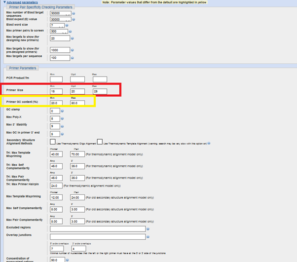
By using advanced parameters, you can optimize the “primer size” and “Primer GC content (I prefer 40-60 for GC content and, 18-20-23 for primer length. Please keep in mind that the efficiency of the primers might change depending on the difference between GC-AT ratio due to difference between the hydrogen bond number, 3 for G-Cs. 2 for A-T.)

Let’s wait little bit after the submission.

In the next window, you will see the region your primer pairs will be amplifying. You will also see the details of the primer pairs (e.g. annealing temperature, whether there is self-complementarity or not).

The black boxed are exons. The yellow box shows the exon-exon spanning region. The red one shows the protein coding region (not every transcripts encodes for protein).

The blue arrows in pair show the primer pair that fits to the parameters we selected on the target.

Please keep in mind that we do not want to select the 3′ end of the transcript (rightmost region) due to RNA degradation characteristics. Particularly 3′ end was effected more in this case. 5′ end might be safer (leftmost).

Even if they seem okay, we need to look them in detail.

When we look at the report, you will see that the target length is 162 (in between ideal, 100-200). Exon-exon spanning. Primer lengths are ideal, too: 19 and 20. Tm is around 60<=. GC ratio is okay: 40-60%. There is little bit the possibility of self-complementarity, unwanted primer dimers, however might be in the acceptable range.

On the other hand, if it targets other variants or other genes than the target, then there is an issue. Unfortunately, we see other regions can be amplified in addition to the target. If this is confirmed by in silico PCR, this means there pairs are not specific enough an whereby not suitable.

In this case, an alternative tool might be useful. For example, Primer3.

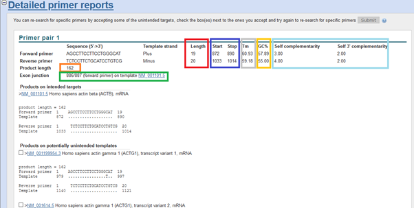
When we look at the report, you will see that the target length is 162 (in between ideal, 100-200). Exon-exon spanning. Primer lengths are ideal, too: 19 and 20. Tm is around 60<=. GC ratio is okay: 40-60%. There is little bit the possibility of self-complementarity, unwanted primer dimers, however might be in the acceptable range.

On the other hand, if it targets other variants or other genes than the target, then there is an issue. Unfortunately, we see other regions can be amplified in addition to the target. If this is confirmed by in silico PCR, this means there pairs are not specific enough an whereby not suitable.

In this case, an alternative tool might be useful. For example, Primer3.

Primer3

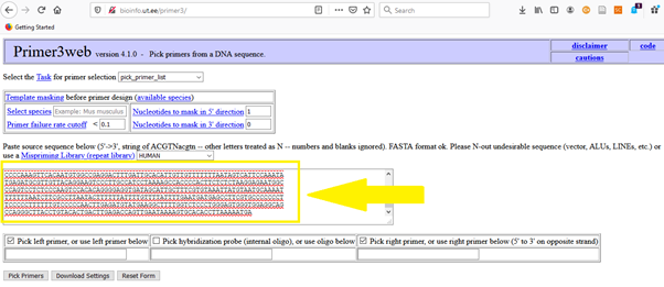
The home page of Primer3 is here. As a next step, just copy and paste the FASTA sequence from NCBI for the target gene you want to amplify. For ACTB, it is here.

Here, you have similar parameters (e.g. primer size, target size, GC %, minimum-maximum Tm) that you can play with.

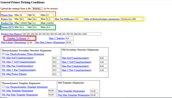
Click “pick primers” after adjusting the parameters based on your need:

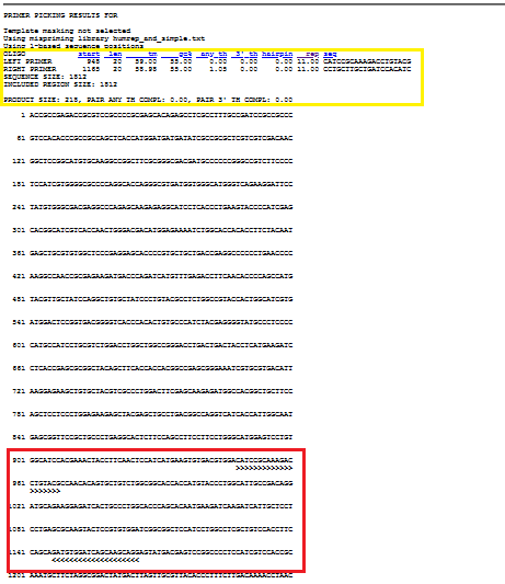
In the yellow box, you see the details of the primer pair, while red box show where it amplifies.

When you scroll down, you can see 9 primer pair candidates that suit with the parameters.

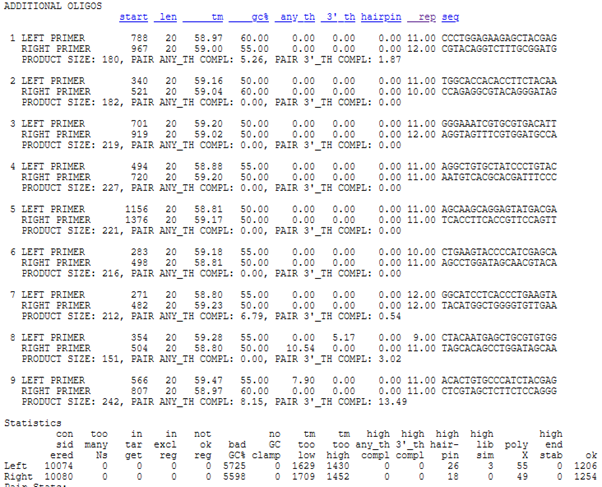
It would be better to choose primer pairs closer to left side (if you do not have any specific aim requiring the 3’end of it) due the reasons explained above. Let’s choose the second alternative in 100-200nt target range ( 1.and 8. can be alternatives, if 2. is not a good candidate).

Then, we will use In silico PCR to confirm.

In silico PCR

Before setting up qPCR for the primers or ordering them for qPCR, it is better to test them on in silico environment. This enables to see how specific your primers for the target sequence in the latest genome assembly.

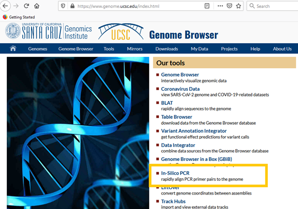
We could not chose the exon-exon spanning option in Primer3. However, it can also be confirmed in silico.

If there is at least one intron between them (namely a longer target than primer3 shows) when you run an agarose gel after q/PCR, it is highly likely due to DNA contamination for RNA samples. Whereas exon-exon spanning regions are composed of transcripts

If the primers are not specific and amplify other sequences than the targets (multiple and non-specific targets), In Silico PCR of UCSC will help you to catch (as a dry-lab tool).

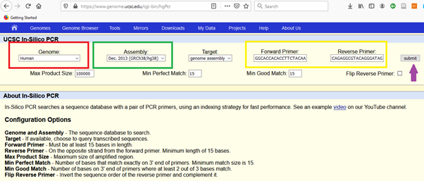
It would be better to choose the latest assembly of human genome for more accurate representation. Then copy and paste the forward and reverse primers for the given regions.

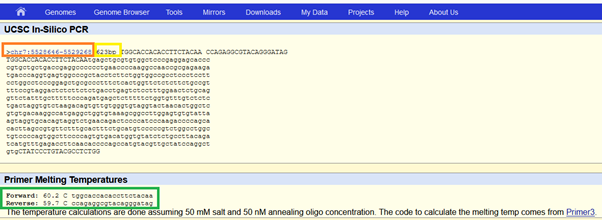
As a result of in silico PCR test, you see that the primers are amplifying a region at chromosome 7, which is the location where ACTB resides. There is also only one amplified target, that is great. Besides, there is at least one intronic region on the genome (it is longer than the target region, 182 vs. 163), which is not in the transcriptome where only exons are available. Therefore, if there is any DNA contamination, and the length of wet-lab PCR product is longer than the target, you can easily spot the difference and the reason.

Reference (Housekeeping) Gene

qPCR is done to measure gene expression. However, there might be changes in the gene expression due to the some intrinsic or technical reasons (e.g. not put equal amounts of material) during the experiments. To rule out any bias in the data, a reference (housekeeping) gene is used. There are the genes that supposed to have similar expression profile no matter the condition, mutation fo the target and time point is.

Having said that, it is important to choose reference gene carefully. They should have similar expression profile among different tissues (if you are comparing a target from different tissues) or not affected by the specific modification (e.g. mutation done on the target.

Actin and GAPDH were chosen historically, independent of the study type. However, recent studies showed that they are not always stable for every tissue or experiment condition. Due to this, there are now different studies helping you to identify most proper reference gene. It is better to keep up the following recent literature.

For example, there is an article, providing the reference gene for each cancer type:

Conventionally used reference genes are not outstanding for normalization of gene expression in human cancer research (suggestions: • HNRNPL • PCBP1 • RER1)

this article also provides good insights regarding how to choose reference gene:

Human housekeeping genes, revisited

qPCR Data Analysis

What do you expect to see when you analyze the qPCR data? Relative expression (e.g. gene A is expressed 10 times more than gene B) or absolute expression (e.g. gene A is expressed this much, whereas gene B is expressed that much)?

There are two common methods for qPCR data analyses (delta methods) suggested by Livak et al.:

• 2^(-𝚫CT)
• 2^(-𝚫𝚫CT

Method 1: [2^(-𝚫𝚫CT)]

In this method, we first normalize the target (GBGT1l3) using the reference (ACTB). As a next step, the unhealthy expression (Ct) is normalized to healthy, also shown as calibrator, expression (Ct). Then, you will find the relative expression as a fold-change.

𝚫CT (calibrator) = 𝚫CT(gbgt1l3) – 𝚫CT(b-actin)

𝚫CT (calibrator) =  17-18 = -1.0

𝚫CT (disease) = 𝚫CT(gbgt1l3) -𝚫CT (b-actin)

𝚫CT (disease) = 14-19 = -5

𝚫𝚫CT= 𝚫CT(disease) -𝚫CT(calibrator)

𝚫𝚫CT= -5 – (-1) = -4

2^(-𝚫𝚫CT)= Normalized expression = 2^(-4) = 16

What does it mean? gbgt1l3 gene is expressed 16 times more in diseased condition compared to healthy individuals.

Method 2: [2^(-𝚫CT)]

In this method, we first find the relative expression of the relevant genes (i.e. gbgt1l3 vs. bactin) in the condition (i.e. healhty, diseased).

2^(𝚫CT of bactin – 𝚫CT  of gbgt1l3) = Find relative expression

For calibrator = 2^(𝚫CT of bactin – 𝚫CT  of gbgt1l3) = 2^(18-17) =21=2

For disease= 2^(𝚫CT of bactin – 𝚫CT  of gbgt1l3) =2^( 19-14) =25= 32

Then, find the expression corresponding these:

Healthy = calibrator/calibrator=2/2=1

Disease = Disease/ calibrator= 32/2=16 times more gbgt1l3 expression.

Additional Notes

Gene Expression in Different Tissues

To learn which genes are expressed in which tissues and how much expressed, these online tools might help you to find out quickly: GeneCards and ExpressionAtlas.

Primer Efficiency Calculation

Apart from the calculations above, there are other measurement that primer efficiency is taken into consideration.

Lets first understand what “PCR efficiency” means. The primers that matches with the target regions are supposed to double in every cycle to be amplified. However, we do not really know whether this is the case or not. In the above calculations, we assumed that it is the case. In case, you wonder how efficient the primers in the given PCR conditions are, you can test them by serial dilutions of cDNA.

If you reduce the amount of the cDNA to its half, the material that PCR amplifying will be reduced to its half. For every dilution, PCR will reach threshold expression value (denoted as Ct) later. When you put the Ct values on a graph in Excel or GraphPad, you will get a line. This line shows how efficient your primers are.

R: correlation. If correlation value is near to +/-1, this shows that primers are effectively doubled in every cycle as expected.

Why log? Because,

 log2(2) =1 

 log2(4)=2 

 log2(1/2)= -1

 log2(1/4)=-2 

….

Whenever it is doubled, you can get a fold-change in a proper value in log base. When it is half, -1 fold-change, when it is doubled, +1 fold-change etc. Briefly, log provides you a straight correlation line for the situations of increment/decrement.

Acknowledgements

I would like to thank my master thesis supervisor Dr. Ozlen Konu, and my dear friends (particularly Ayse Gokce Keskus, Said Tiryaki, and Seniye Targen) from KONU Lab who shared their experience/knowledge with me during the beginning of my academic life while practicing the basics of the bioinformatics and wet-lab.

References

• Turkish version of this post: https://rsgturkey.com/tr/primer-dizayna-giris-tutorial-101/ (by Fatma Betül Dinçaslan)
• A Nobel winning method: PCR: : https://www.nobelprize.org/prizes/chemistry/1993/mullis/lecture/
• PCR and COVID: https://my.clevelandclinic.org/health/diagnostics/21462-covid-19-and-pcr-testing
• NCBI website: https://www.ncbi.nlm.nih.gov/
• Ortholog vs Paralog: Jensen, R.A. Orthologs and paralogs – we need to get it right. Genome Biol 2, interactions1002.1 (2001). https://doi-org.libproxy1.nus.edu.sg/10.1186/gb-2001-2-8-interactions1002
• Exon-exon junction: https://sg.idtdna.com/pages/education/decoded/article/use-splice-junctions-to-your-advantage-in-qpcr
• Primer3: http://bioinfo.ut.ee/primer3/
• UCSC: https://www.genome.ucsc.edu/index.html
• In silico PCR: https://www.genome.ucsc.edu/cgi-bin/hgPcrEisenberg E, Levanon EY.
• Human housekeeping genes, revisited [published correction appears in Trends Genet. 2014 Mar;30(3):119-20]. Trends Genet. 2013;29(10):569-574. doi:10.1016/j.tig.2013.05.010Jo, J., Choi, S., Oh, J. et al.
• Conventionally used reference genes are not outstanding for normalization of gene expression in human cancer research. BMC Bioinformatics 20, 245 (2019). https://doi-org/10.1186/s12859-019-2809-2
• qPCR analysis: Livak KJ, Schmittgen TD. Analysis of relative gene expression data using real-time quantitative PCR and the 2(-Delta Delta C(T)) Method. Methods. 2001;25(4):402-408. doi:10.1006/meth.2001.1262
• Gene Cards: https://www.genecards.org/
• Expression Atlas: https://www.ebi.ac.uk/gxa/home
• Primer Efficiency Calculation: http://www.sigmaaldrich.com/technical-documents/protocols/biology/qpcr-efficiency-determination.html
• An example graph about how to evaluate the efficiency of qPCR: https://www.novusbio.com/products/afm-primer_nbp1-71653vusbio.com/products/afm-primer_nbp1-71653